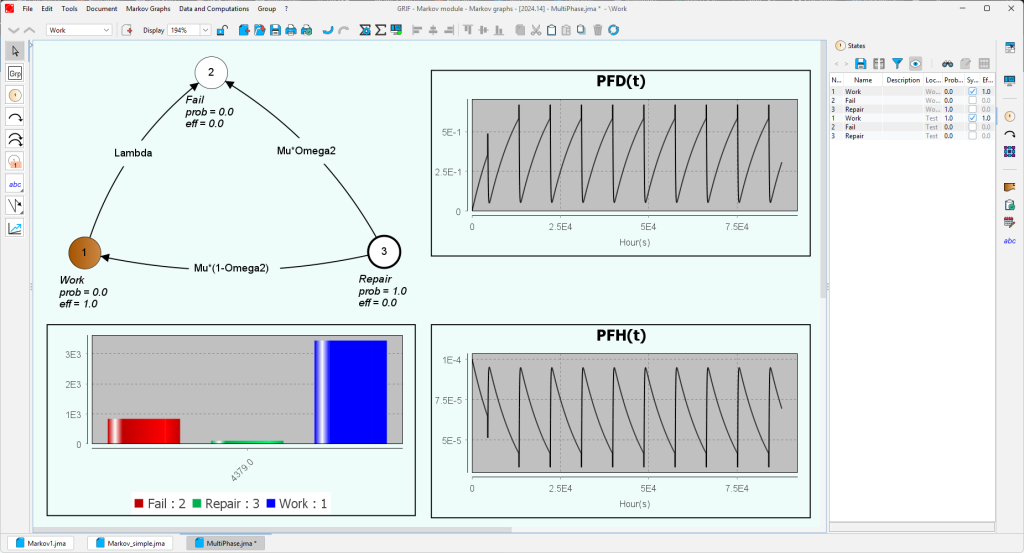
As its name suggests, this package lets you model Markov graphs. It consists of the Markovian module. Its computational algorithm enables it to handle graphs with several hundred states without any problem.
This package can handle systems with temporal dependencies (one event must occur before another) or a limited number of repairers. By its very nature, it represents all possible states of the element under study. On its own, it is therefore mainly used for small systems/equipment.
In addition to the usual times spent in the various states and the probabilities of being in a state, the Markov module also computes the system’s failure rate.

Multi-Phase Markov
Industrial systems do not necessarily behave in the same way throughout their lifetime. Whether in summer/winter, storage/operation or maintenance/production phases, a single Markov graph is often unable to model the system.
This is why the Markov module allows you to define several graphs, each corresponding to a phase in the life of the system. The Markov module can then perform a multi-phase Markov computation by concatenating the different graphs.


FT Driven Markov Graph
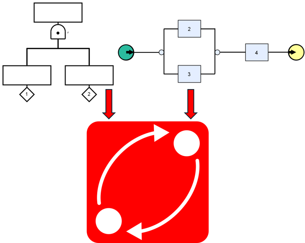
Coupled with the Boolean package, the Markov module lets you take full advantage of Fault-Tree driven Markov Graph, and Reliability Block Diagram driven Markov Graph. These modeling methods enable you to create independent Markov Graphs for individual devices, then assemble them into a higher-level Boolean model.
If your system is 99% static, apart from the 1oo2 power supply system itself, which is backed up by a generator, the urge to create a fault tree is strong. But the power supply part can’t be modeled correctly by a Boolean approach, and that’s where FT driven Markov Graphs come into their own.
